41 how to make a diagram in excel

How to Make Charts and Graphs in Excel | Smartsheet Excel provides Recommended Charts based on popularity, but you can click any of the dropdown menus to select a different template. Step 2: Create Your Chart From the Insert tab, click the column chart icon and select Clustered Column. Excel will automatically create a clustered chart column from your selected data. How to Create a Graph in Excel: 12 Steps (with ... - wikiHow You can create a graph from data in both the Windows and the Mac versions of Microsoft Excel. Steps 1 Open Microsoft Excel. Its app icon resembles a green box with a white "X" on it. 2 Click Blank workbook. It's a white box in the upper-left side of the window. 3 Consider the type of graph you want to make.

Create a Pareto Chart in Excel (In Easy Steps) If you don't have Excel 2016 or later, simply create a Pareto chart by combining a column chart and a line graph. This method works with all versions of Excel. 1. First, select a number in column B. 2. Next, sort your data in descending order. On the Data tab, in the Sort & Filter group, click ZA. 3. Calculate the cumulative count.

How to make a diagram in excel

Create a waterfall chart - support.microsoft.com Create a waterfall chart. Select your data. Click Insert > Insert Waterfall or Stock chart > Waterfall. You can also use the All Charts tab in Recommended Charts to create a waterfall chart. Tip: Use the Design and Format tabs to customize the look of your chart. If you don't see these tabs, click anywhere in the waterfall chart to add the ... How to Make a Sankey Diagram Excel Dashboard? In 3 Easy Steps Creating a Sankey diagram in Excel is very easy if you break the process into these three steps: Generate data for all individual Sankey lines. Plot each individual Sankey line seperately. Assemble all individual Sankey lines together into a Sankey diagram. I'll show you how each one of these steps work in greater detail. How To Make A Waterfall Bridge In Excel? | kyinbridges.com Step 2: Make Excel bridge diagrams based on stacked columns. How Do You Create A Stacked Waterfall Chart In Excel? Ensure that the data range is selected. Using the up slide ribbon, click the drop-down menu for the Charts tab. To access Waterfall, click on the CTRL+Shift+B key combination.

How to make a diagram in excel. How to Make a Basic Gantt Chart in Excel Make a Gantt Chart in Excel to Track Your Projects. You can manage your projects by creating a Gantt chart in Excel. If it's a small, one-off event, you can make a simple Gantt chart by using the first method discussed above. If it's a more complicated, elaborate project, you'll find that Gantt chart templates are more suitable. How to Create Visio Diagram from Excel | Edraw - Edrawsoft Launch Microsoft Excel, go to Insert, click the small triangle available next to the My Add-ins option in the Add-ins group, and click Microsoft Visio Data Visualizer to launch the add-in. Step 2: Create a Visio Diagram Select a category from the left section of the Data Visualizer box, and click your preferred diagram from the right. How to Create a Gauge Chart in Excel? - GeeksforGeeks Steps to Create a Guage Chart. Follow the below steps to create a Gauge chart: Step 1: First enter the data points and values. Step 2: Doughnut chart (with First table values). Select the range B2:B7. Then press shortcut keys [Alt + N + Q and select the Doughnut] or Go to Insert -> Charts -> Doughnut (With these steps you will get a blank chart). How to Create an Excel Map Chart from Pivot Data? 3 Simple ... Step 1: Copy the Pivot table data. The solution is to remove the data from Pivot Table first and then create the map chart. Click in the PivotTable and press Ctrl+A to select all the data. Click in a blank cell somewhere else in the worksheet. From the Home tab, in the Clipboard group, click the lower-half of the Paste button.

Create a diagram in Excel with the Visio Data Visualizer ... If you're not signed in, then the diagram is part of your Excel workbook instead. You can always choose to create a Visio file by signing in. To create your own diagram, modify the values in the data table. For example, you can change the shape text that will appear, the shape types, and more by changing the values in the data table. How to make Gantt chart in Excel (step-by-step guidance ... 2. Make a standard Excel Bar chart based on Start date. You begin making your Gantt chart in Excel by setting up a usual Stacked Bar chart. Select a range of your Start Dates with the column header, it's B1:B11 in our case. Be sure to select only the cells with data, and not the entire column. Switch to the Insert tab > Charts group and click Bar. Exactly how to Make a Bar Chart in Microsoft Excel ... When your information is selected, click Insert > > Insert Column or Bar Chart. Various column charts are offered, yet to insert a typical bar graph, click the "Clustered Chart" alternative. This graph is the very first symbol noted under the "2-D Column" section. Excel will automatically take the data from your data set to produce the ... How to Create a Fishbone Diagram in Excel | EdrawMax Online Go to Insert tab, click Shape, choose the corresponding shapes in the drop-down list and add them onto the worksheet. c. Add Lines Go to Insert tab or select a shape, go to Format tab, choose Lines from the shape gallery and add lines into the diagram. After adding lines, the main structure of the fishbone diagram will be outlined. d. Add Text

How to plot a ternary diagram in Excel Insert a Scatter Chart (XY diagram), e.g., 'Scatter with Straight Lines' (Figure 9) using the XY coordinates for the triangle from columns AA and AB. To make it into an equilateral triangle resize the chart area accordingly; for example 10 columns wide and 30 rows high, as in Figure 10. Create a Line Chart in Excel (In Easy Steps) - Excel Easy To create a line chart, execute the following steps. 1. Select the range A1:D7. 2. On the Insert tab, in the Charts group, click the Line symbol. 3. Click Line with Markers. Result: Note: only if you have numeric labels, empty cell A1 before you create the line chart. How to Create Venn Diagram in Excel - Free Template ... Step #1 - Calculate Chart Values: Type "=B2-B5-B6+B8" into cell D2. Type "=B3-B5-B7+B8" into cell D3. Type "=B4-B6-B7+B8" into cell D4. Step #2 - Calculate Chart Values cont.: Enter "=B5-$B$8" into D5 and copy the formula down into D6 and D7. Step #3 - Calculate Chart Values cont.: Set cell D8 equal to B8 by typing "=B8" into D8. How To Create A Gantt Chart In Excel - Thisisguernsey.com Here's how you can create an Excel timeline chart using SmartArt. Click on the Insert tab on the overhead task pane. Select Insert a SmartArt Graphic tool. Under this, choose the Process option. Find the Basic Timeline chart type and click on it. Edit the text in the text pane to reflect your project timeline.

Create a Pie Chart in Excel (In Easy Steps) - Excel Easy Pie charts are used to display the contribution of each value (slice) to a total (pie). Pie charts always use one data series. To create a pie chart of the 2017 data series, execute the following steps. 1. Select the range A1:D2. 2. On the Insert tab, in the Charts group, click the Pie symbol. 3. Click Pie.

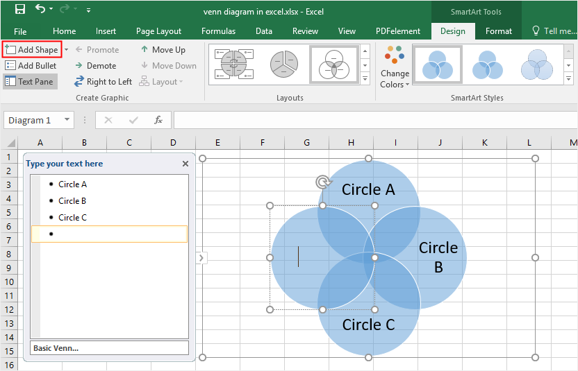
How to Create Venn Diagram in Excel? - EDUCBA Now the following steps can be used to create a Venn diagram for the same in Excel. Click on the 'Insert' tab and then click on 'SmartArt' in the 'Illustrations' group as follows: Now click on 'Relationship' in the new window and then select a Venn diagram layout (Basic Venn) and click 'OK.

Create a Sankey diagram in Excel - Excel Off The Grid It just needs each column category from the source data listed with a "Blank" item in between. The formula for the Value is: =SUMIFS (SankeyLines [Value],SankeyLines [To], [@To]) Spacing named range The final part of the interim calculations is a named range called Spacing. This is used as the Category (horizontal) Axis for the chart.

How to Make a Graph in Excel: A Step by Step Detailed Tutorial Create the Basic Excel Graph. With the columns selected, visit the Insert tab and choose the option 2D Line Graph. You will immediately see a graph appear below your data values. Sometimes if you do not assign the right data type to your columns in the first step, the graph may not show in a way that you want it to.

How to Create a Sankey Diagram in Excel Spreadsheet Excel spreadsheet does NOT have Sankey templates. To create a Sankey chart in Excel, start by installing an external ChartExpo Add-in. And then, browse to find the Sankey chart. It's the first chart in ChartExpo's ultra-friendly user interface. Use this chart to visualize flows and processes in business settings.

Create a Map chart in Excel - support.microsoft.com Just click on the map, then choose from the Chart Design or Format tabs in the ribbon. You can also double-click the chart to launch the Format Object Task Pane, which will appear on the right-hand side of the Excel window. This will also expose the map chart specific Series options (see below).

How to Make a Burndown Chart in Excel | Nifty Blog To ask Excel to create the graph or the burndown chart, you should follow these steps: Select the three right columns of 'Dates,' 'Planned,' and 'Actual.'. In the top menu bar, select Insert. Select the line chart icon from the drop-down menu. Choose a basic line chart from the menu.

How To Make A Fishbone Diagram In Excel - Studying Diagrams Here well show how to make such a diagram in Excel How to Create a Fishbone Diagram Step 1. Select a format xlsx. Well begin by constructing the main arrow in the middle of the fishbone diagram. Select a rectangle from the shape library and add it to the correct side of your slide. A Fishbone diagram is also called cause-and-effect diagramThe ...

How To Make A Waterfall Bridge In Excel? | kyinbridges.com Step 2: Make Excel bridge diagrams based on stacked columns. How Do You Create A Stacked Waterfall Chart In Excel? Ensure that the data range is selected. Using the up slide ribbon, click the drop-down menu for the Charts tab. To access Waterfall, click on the CTRL+Shift+B key combination.

How to Make a Sankey Diagram Excel Dashboard? In 3 Easy Steps Creating a Sankey diagram in Excel is very easy if you break the process into these three steps: Generate data for all individual Sankey lines. Plot each individual Sankey line seperately. Assemble all individual Sankey lines together into a Sankey diagram. I'll show you how each one of these steps work in greater detail.

Create a waterfall chart - support.microsoft.com Create a waterfall chart. Select your data. Click Insert > Insert Waterfall or Stock chart > Waterfall. You can also use the All Charts tab in Recommended Charts to create a waterfall chart. Tip: Use the Design and Format tabs to customize the look of your chart. If you don't see these tabs, click anywhere in the waterfall chart to add the ...

Share this post